We estimate here the evolution rate for the Quasispecies model, which describes the
evolution of informational sequences population {Sk}
, k = 1,..., n. The sequence symbols are taken
from an alphabet, containing l letters,
the sequence length equals to N . The evolution process
consists of consequent generations, which include selection and
mutations of the sequences Sk
.
We consider the stochastic case (lN >> n) under the
following simplifying assumptions:
| ; |
1) the alphabet consists of two letters (l = 2), namely, sequence
symbols take the values: Ski
= 1, -1; k = 1,..., n ; i =
1,..., N ; |
| ; |
2) the selective value of any sequence S is
defined as: |
| |
f(S)
= exp[-b r(S,Sm)], |
(1) |
| |
where b is a
selection intensity parameter, r(S,Sm) is the
Hamming distance between the given sequence S
and the master sequence Sm ; |
| |
3) the mutation intensity P , that is the
probability to reverse a sign of any symbol (Ski
--> - Ski)
during mutations, is sufficiently small: |
| |
PN  b,
1. b,
1. |
(2) |
Note, that for large P , the already found
"good" sequences could be lost, so the inequality (2)
is a condition for the successful evolutionary search of the
sequences with large selective values (see [1,2] for details).
The inequality (2) implies also a rather large selection
intensity.
In addition, we assume that the population size n is
sufficiently large, so a neutral selection effect [3] can be
neglected (see below for the more detailed consideration).
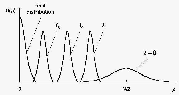
Fig. 1 illustrates schematically the sequence distribution
dynamics during the evolution process. Here n(r) is the number of
sequences S , such that r(S,Sm) = r
in a considered population; t is the generation number.

Fig. 1. The sequence distribution n(r) at
different generations t ; t3 > t2
> t1 (schematically, according to the
computer simulations [2]).
The initial sequence distribution (t = 0) is a random
one, it spreads in the vicinity of the value r0 = N/2 (r0
is the mean distance between an arbitrary sequence S
and the master one Sm).
The sequences with small r ,
having large selective values, are absent in the initial
population. At the first several generations, the sequences,
having maximal available in initial population selective value
(corresponding to the left edge of the distribution at t
= 0), are quickly selected, and the distribution becomes more
narrow than the initial one. Such a distribution is shown in
Fig.1 by the curve at t1 .
At further generations the distribution is shifted to the left
(the curves at t2 , t3)
until the final distribution (placed near r
= 0) is reached. Because the selection intensity b is rather large (see (2)), the
"shift" process is limited mainly by mutations.
Typically of the order of dt
= (PN)-1 generations (dt
is typical time for one mutation per sequence) are needed to
shift the distribution to the left on the value dr = 1. So, we can estimate the
total number of evolution generations by the value
| T ~ dt
x (N/2)/dr
~ (N/2)x(PN)-1. |
(3) |
Eq. (3) characterizes roughly the evolution rate.
So far we have neglected the neutral selection effect, which
is essential at a small population size [3]. The neutral
selection is the random fixation in a population an arbitrary
"species", regardless of a selective value. It could
suppress the search of the "good" sequences. Typical
time Tn of neutral selection is of
the order of a population size n (see Neutral evolution game for details). We
can neglect the neutral selection, if the total generation number
T is smaller than Tn :
The inequality (4) is a condition, at which the estimation of
the evolution rate (3) is valid.
In addition, we can construct the "optimal"
evolution process, which involves the minimal total number of
participants ntotal = nT under
condition that master sequence is found. The "optimal"
evolution corresponds to the maximal permissible mutation
intensity P ~ N -1 (see (2)). At
this P , according to (3), we have T ~ (N/2)
. Taking into account (4), we can set n ~ 2N and
obtain finally:
The estimation (5) characterizes the
effectiveness of the evolution process as an algorithm for search
of the optimal (master) sequence.
The estimations (3), (5) were confirmed by
computer simulations [2].
References:
1. M.Eigen, P.Schuster. "The
hypercycle: A principle of natural self-organization".
Springer Verlag: Berlin etc. 1979.
2. V.G.Red'ko. Biofizika. 1986. Vol. 31.
N.3. P. 511. V.G.Red'ko. Biofizika. 1990. Vol. 35. N.5.
P. 831 (In Russian).
3. M. Kimura. "The neutral theory
of molecular evolution". Cambridge Un-ty Press. 1983.

